
How to Analyze a $2M Multifamily Deal: A Hypothetical Walkthrough
Part of the Multifamily Investing guide.
The short answer
This is a hypothetical educational example created by DealWorthIt. The property, its operating history, the financing assumptions, the investor and the results are all illustrative. They do not describe an actual customer or an actual transaction, and they are not a promise of performance. Every figure below was invented to teach a method; none of it is a market benchmark, a loan quote, or a projection of what your deal will do.
Underwriting a $2,000,000 multifamily property means rebuilding the seller's income and expenses from primary documents, testing what a lender will actually lend against them, projecting operations you can defend, and then deciding whether the price clears the return you require. The order matters, because each step constrains the next: the rent roll sets the income, the income sets the NOI, the NOI sets the loan, the loan sets the equity, and the equity sets the return. If you want the method without a worked example attached, the step-by-step guide to underwriting a multifamily deal covers the same sequence in general terms.
Worked end to end on the hypothetical property below, that process produces this: an in-place net operating income of $97,941, a going-in cap rate of 4.90% at a $2,000,000 price, a loan that sizes to $945,000 rather than the $1,300,000 the buyer asked for, an equity requirement of $1,484,450, a five-year levered IRR of 4.3% and an equity multiple of 1.22x.
Under these hypothetical assumptions the calculation produces a deal that fails four of the six example targets set later in this article. That is the useful part. The point of underwriting is not to reach a number that justifies an offer already decided on — it is to find out what price, if any, the property supports. This one supports about $1,215,066 against the full target set, not $2,000,000.
Change the price, the rents, the vacancy, the expenses, the interest rate, the capital budget or the exit cap rate and every one of those results moves. The stress tests in Step 9 show by how much.
What this walkthrough is, and what it is not
It is a complete, reproducible underwriting method applied to an invented property, using capabilities that exist in DealWorthIt today. Every displayed figure can be re-derived from the assumptions printed on this page — that is the standard this article is held to, and it is enforced by an automated check that recomputes the whole model from those assumptions each time the site is built.
It is not any of the following, and it is worth being explicit because articles in this genre routinely are:
- Not a customer story. No investor wrote this, no investor is quoted in it, and no customer outcome is being reported. DealWorthIt wrote it.
- Not a real transaction. The property does not exist. The address, the seller, the broker and the lender are all absent because there are none.
- Not a speed claim. How long an analysis takes depends on the quality of the documents you receive and how much of the seller's reporting you have to rebuild. This article makes no claim about elapsed time, and you should be skeptical of any that does.
- Not market data. The rents, expenses, cap rates and loan terms here were chosen to make a teaching example work, not to represent any market. Where you need real benchmarks, the sources are listed at the end.
- Not advice. Nothing here is investment, tax, legal or lending advice, and no software — DealWorthIt included — can tell you whether a property is a suitable investment for you.
The hypothetical property and acquisition
Everything in this section is invented. It describes a 1978-vintage garden-style property in an unnamed secondary market, listed at exactly $2,000,000 as a value-add opportunity: below-market rents, three vacant units, and a deferred-maintenance list the seller has been putting off.
| Unit type | Units | Occupied | Size | In-place rent | Market rent |
|---|---|---|---|---|---|
| 1 bed / 1 bath | 8 | 7 | 650 sf | $845/mo | $925/mo |
| 2 bed / 1 bath | 14 | 12 | 875 sf | $985/mo | $1,095/mo |
| 3 bed / 2 bath | 2 | 2 | 1,050 sf | $1,150/mo | $1,295/mo |
| Total | 24 | 21 | — | — | — |
Physical occupancy is 87.5% — 21 of 24 units. Property age is 48 years. The seller has an aging-report list of deferred items and no capital plan. There is no on-site staff beyond a part-time caretaker, and the seller manages the property personally without charging a management fee to the T12 — a detail that matters enormously in Step 2.
The market is deliberately unnamed. Naming a real city would invite you to read invented rents as that city's rents, and they are not.
Step 1: Read the rent roll
The rent roll is the only document that tells you what is actually being collected, unit by unit, today. It is also the document sellers most often present in its most flattering form. Start by separating four things the summary line tends to blend together.
| Line | Amount | How it is calculated |
|---|---|---|
| Gross potential rent | $303,840 | Every unit at its market rent, twelve months, whether or not it is occupied. |
| In-place scheduled rent | $240,420 | Occupied units only, at the rent each lease actually says. |
| Less loss to lease | −$26,040 | Occupied units, market rent less lease rent. This is rent you are not collecting from tenants who are already there. |
| Less vacancy | −$37,380 | The three vacant units, valued at market rent. |
| Less concessions | −$6,000 | Free-rent and move-in incentives granted on recent leases. |
| Less credit loss and delinquency | −$4,300 | Billed rent that was never collected. |
| Effective rental income | $230,120 | What the rent roll and the ledger together say the property collects. |
Two occupancy figures fall out of this, and confusing them is one of the more expensive mistakes in multifamily. Physical occupancy is 87.5% — a count of doors. Economic occupancy is 75.7% — effective rental income divided by gross potential rent. The 11.8-point gap is the loss to lease, the concessions and the delinquency. A property can be 95% physically occupied and still collect badly.
Because different people define economic occupancy differently, this article states its convention rather than assuming yours: loss to lease is included in the drag. If you exclude it and measure collections only against vacancy, concessions and credit loss, the same rent roll reads 84.3%. Neither is wrong; publishing one without saying which is.
Note also that physical vacancy of 12.5% (3 of 24 doors) produces a 12.3% revenue vacancy, because the vacant units are not the most expensive ones. Unit counts and dollars are not interchangeable.
Beyond the arithmetic, a rent roll review should answer questions no total will surface for you. Each of these is expanded on in the guide to what investors should check in a rent roll before making an offer:
- Occupied versus leased. A unit can be leased and not yet occupied, or occupied by someone who is not on the lease. Both distort a rent roll.
- Lease expirations. How many leases roll in the first ninety days after closing? A concentration of expirations is either an opportunity to reprice or a vacancy cliff, depending on the market and your make-ready capacity.
- Month-to-month tenancies. Flexible for repricing, unstable for occupancy, and in some jurisdictions subject to different notice rules than a term lease.
- Concessions. Whether they are one-time or recurring changes their treatment. A concession granted on every renewal is a rent reduction wearing a disguise.
- Delinquency by unit. A single unit that is four months behind is a very different problem from twelve units that are each a week late.
- Employee and model units. Units occupied by staff or used as a leasing office produce no rent and are often quietly counted as occupied.
- Down units. A unit that cannot be leased until it is repaired is not vacancy, it is capital expenditure. Verify which of the three vacant units here are rent-ready.
- Unit mix versus the market. Two three-bedroom units in a submarket that rents mostly to single occupants is a different exposure than the door count suggests.
- Loss to lease, unit by unit. An average conceals whether the gap is one badly-priced unit or the whole property.
Step 2: Normalize the T12
The trailing twelve-month statement records what the seller spent. Underwriting requires what you will spend, which is a different number for reasons that are mostly predictable. Normalizing means adjusting each line to your ownership, and documenting every adjustment so a lender or a partner can follow the reasoning.
Two lines in this example move materially, and both are the kind that get missed.
| Line | Seller's T12 | Underwritten | Why it changes |
|---|---|---|---|
| Property taxes | $19,800 | $29,000 | The assessment reflects the seller's basis, not yours. This example assumes reassessment at the purchase price at a 1.45% effective rate — an invented rate. Reassessment rules vary enormously by state and county, and getting this wrong is worth more than most negotiating wins. |
| Insurance | $13,100 | $17,400 | The seller's policy is not your policy. This uses a hypothetical quoted renewal, which is what you should be underwriting to — not last year's premium. |
| Property management | $0 | $12,207 | The seller self-manages and charges nothing. A buyer must underwrite the market cost of management even when planning to self-manage, because the labor is real and because a lender will impute it. |
| Repairs and maintenance | $8,900 | $13,200 | A 48-year-old property that has been deferring work does not spend $371 per unit per year sustainably. Underwritten at $550 per unit. |
| Payroll | Not stated | $26,400 | The seller's personal labor appears nowhere. Someone has to do the work after closing. |
The general discipline, beyond these five lines — and the companion guide to analyzing a T12 statement before buying works through each of them against a full operating statement:
- Separate recurring from non-recurring income. A lease-break fee, an insurance settlement or a one-time utility refund is not income you can capitalize.
- Separate recurring expenses from capital. A roof is not repairs and maintenance. If the seller ran capital work through the operating statement, NOI is understated; if they ran repairs through capital, it is overstated. Both happen, and they happen in the direction that flatters the seller.
- Look for what is missing. Absent lines are harder to spot than wrong ones. Management, payroll, replacement reserves, snow removal in a market that gets snow — a T12 that lacks a line does not mean the cost does not exist.
- Check utility trends month by month. An annual total hides a leak. Rising water expense with flat occupancy is a plumbing problem you are about to buy.
- Ask what changed mid-year. A contract renegotiated in month nine means the T12 understates the run rate by three-quarters of the increase.
- Normalize, do not smooth. If a line is genuinely volatile, underwrite the level you can defend and say so, rather than averaging away the risk.
Step 3: Calculate in-place NOI
Before the arithmetic, the convention — because NOI is not one number, and three different people at the same closing table will each mean something slightly different by it.
| Item | Treatment here | Why |
|---|---|---|
| Operating expenses, including property management | Above NOI | They are the cost of running the property at its current revenue. The management fee is charged on effective gross income, so it moves with revenue. |
| Property taxes, reassessed | Above NOI | Reassessed at the hypothetical purchase price. Using the seller's assessment would overstate NOI by $9,200 in this example. |
| Replacement reserves | Below NOI | They fund recurring capital — appliances, flooring, HVAC — not operations. Reported separately so the lender basis can net them out. |
| Capital expenditure | Excluded from NOI | Funded from equity at closing, not from operations. It reaches the return through the equity requirement instead. |
| Debt service | Excluded from NOI | NOI is a property-level measure. It does not know how you financed the purchase. |
| Sponsor asset-management fee | None modeled | This example has no syndication layer. Where one exists, it sits below NOI. |
With that stated, the build-up. Other income is modeled flat at the trailing-twelve level rather than grossed up to full occupancy, which is the conservative choice.
| Income line | Annual |
|---|---|
| Effective rental income (Step 1) | $230,120 |
| Utility reimbursement (water/sewer bill-back) | $6,048 |
| Laundry | $2,880 |
| Pet rent and pet fees | $2,160 |
| Parking and storage | $1,800 |
| Late fees and administrative charges | $1,140 |
| Effective gross income | $244,148 |
| Operating expense | Annual |
|---|---|
| Property taxes (reassessed at 1.45% of $2,000,000) | $29,000 |
| Insurance | $17,400 |
| Payroll (on-site and maintenance) | $26,400 |
| Repairs and maintenance | $13,200 |
| Turnover and make-ready | $9,600 |
| Utilities (owner-paid) | $19,200 |
| Contract services (landscaping, snow, pest, trash) | $10,800 |
| Administrative | $5,400 |
| Marketing and leasing | $3,000 |
| Property management fee (5.0% of effective gross income) | $12,207 |
| Total operating expenses | $146,207 |
That is an operating expense ratio of 59.9% of effective gross income, or $6,092 per unit per year. Both cross-checks are worth doing every time: a ratio that looks normal can still hide a per-unit figure that is impossible for the vintage, and vice versa. Note that the ratio is high partly because the denominator is depressed — the same expenses against stabilized revenue produce a very different ratio, as Step 7 shows.
| Measure | Amount | Definition |
|---|---|---|
| Effective gross income | $244,148 | Effective rental income plus other income. |
| Less operating expenses | −$146,207 | Every line above, including management. |
| Investor-basis NOI | $97,941 | EGI less operating expenses. Reserves are not deducted. |
| Less replacement reserves | −$6,000 | $250 per unit per year, modeled below NOI. |
| Lender-basis NOI | $91,941 | Investor NOI less the replacement reserve. This is the basis the coverage tests in Step 6 use. |
Keep both labeled. Which basis a quoted cap rate or a loan sizing rests on varies by broker, lender, appraiser and transaction — there is no rule you can count on, which is exactly why an unlabeled NOI is a number you cannot safely compare. The $6,000 difference is small here and decisive in thinner deals — and it is the same distinction DealWorthIt draws, which reports the lender basis separately and nets the reserve out of it whenever the reserve is modeled below NOI.
Step 4: Test the price against the cap rate
A cap rate is not a valuation method so much as a way of restating a price as a yield, so that two properties can be compared. Divide NOI by price:
| Basis | NOI | Price | Cap rate |
|---|---|---|---|
| Investor basis | $97,941 | $2,000,000 | 4.90% |
| Lender basis (after reserves) | $91,941 | $2,000,000 | 4.60% |
This article will not tell you whether 4.90% is a good going-in cap rate, because that depends on the market, the vintage, the tenancy, the alternative uses of the capital, and the cost of debt — none of which a hypothetical can supply. What it will say is arithmetic: at $2,000,000 the property costs $83,333 per unit and returns 4.90% on current operations before any debt. Whether that is defensible is a judgment about a real market, made by a person.
The reason a buyer might pay it, of course, is the value-add thesis: 12.5% of the doors are empty and the occupied ones are $26,040 under market. The seller is asking to be paid today for improvements the buyer has to fund and execute. Steps 7 through 10 test whether that trade works.
Step 5: Model the financing
The loan terms below are invented. They are not a quote, not an offer, not an indication of what any lender would do, and not a benchmark. Which loan products a real acquisition of this size could actually reach is a separate question, covered in the overview of multifamily financing options. Where you need real rate context, the U.S. Treasury publishes the daily par yield curve and the New York Fed publishes SOFR — both are cited in the sources at the end, and both are what DealWorthIt itself reads for its benchmark rates.
| Term | Assumption |
|---|---|
| Requested loan-to-value | 65% |
| Requested loan amount | $1,300,000 |
| Interest rate | 6.75%, fixed |
| Amortization | 30 years (360 months) |
| Loan term | 5 years |
| Interest-only period | None |
| Origination fee | 1.00% of the loan |
| Lender third-party costs | $22,000 (appraisal, property condition, environmental, lender legal) |
The monthly payment on a fully-amortizing loan is the loan amount times r* ÷ (1 − (1 + *r)^−n*), where *r is the monthly rate and n* the number of payments. At $1,300,000, 6.75% and 360 months that is *$8,432 a month, or $101,181** a year.
And that is where the requested loan stops being available, which Step 6 explains.
Step 6: Calculate DSCR, debt yield and break-even occupancy
Debt service coverage ratio is NOI divided by annual debt service. It answers: how many times over does the property cover its mortgage? Debt yield is NOI divided by the loan amount. It compares the property's income directly with the size of the loan, independent of the interest rate and the amortization schedule — so unlike DSCR it cannot be flattered by cheap debt or a long amortization. It is a credit-risk ratio, not a return: it does not describe what a lender would actually recover in a foreclosure, which would depend on the costs, the timing and what the property turned out to be worth.
Both are computed here on the lender basis (NOI after replacement reserves), with the investor basis shown alongside so the two are never confused.
| Test | Investor basis | Lender basis |
|---|---|---|
| NOI | $97,941 | $91,941 |
| Annual debt service at $1,300,000 | $101,181 | $101,181 |
| DSCR | 0.97x | 0.91x |
| Debt yield | 7.5% | 7.1% |
A DSCR below 1.00x means the property does not generate enough NOI to make its own mortgage payment. At the requested loan amount this deal does not clear that bar on either basis, and the debt yield is below the 8% level DealWorthIt flags as a guide. The $1,300,000 loan is not available at this price and these operations. This is the single most common surprise in a first underwriting pass, and it is why loan sizing belongs before the pro forma, not after it.
Sizing the loan properly
Lenders size to the smallest of several caps. Using a 1.25x minimum DSCR and an 8% minimum debt yield — both example criteria, discussed in Step 10 — the three caps are:
| Constraint | Maximum loan | How it is derived |
|---|---|---|
| 65% loan-to-value | $1,300,000 | 65% × $2,000,000. |
| 1.25x DSCR | $945,019 | Lender NOI ÷ 1.25 gives the maximum annual debt service, divided by the annual constant per dollar of loan (0.0778 at 6.75% over 360 months). |
| 8% debt yield | $1,149,258 | Lender NOI ÷ 0.08. |
DSCR binds. The loan sizes to $945,000 after rounding down to the nearest thousand — an implied loan-to-value of 47.3%, not 65%. Annual debt service falls to $73,551 ($6,129 a month), lender DSCR lands at exactly 1.25x and lender debt yield at 9.7%.
Note what just happened: the two lender tests now "pass", but only because the loan was shrunk until they did. They are satisfied by construction and say nothing about whether $2,000,000 is the right price. The number that carries the information is the 47.3% loan-to-value — the property can only support about half the debt the buyer wanted, so the buyer has to write a much larger equity check, which is what damages the return in Step 8.
Break-even occupancy
Break-even occupancy asks how far collections can fall before the property stops covering its obligations. It has no single universal definition, so here is this one in full, matching the convention DealWorthIt uses on its deal overview:
- Revenue base: gross potential income — gross potential rent plus other income at its trailing-twelve level. Other income is not grossed up to full occupancy, which makes the result slightly conservative.
- Expenses: every operating expense is treated as fixed at its modeled dollar amount, including the management fee. Treating the management fee and turnover costs as variable would lower the break-even.
- Reserves: reported both ways, because reasonable people differ.
- Debt service: included.
- Result type: this is an economic break-even, expressed as a share of gross potential income. It is deliberately not converted into a number of occupied units: rents differ by unit type, so no single door count corresponds to it, and any that is quoted depends on which units you assume empty first.
| Measure | At the $945,000 loan | At the requested $1,300,000 loan |
|---|---|---|
| Gross potential income | $317,868 | $317,868 |
| Break-even including reserves | 71.0% | 79.7% |
| Break-even excluding reserves | 69.1% | 77.8% |
| Current collections on the same base | 76.8% | 76.8% |
| Cushion | 5.8 points | Negative — the property is already below break-even |
This is the clearest single illustration of what leverage does. The same property, the same operations, the same expenses: at 47.3% loan-to-value there are 5.8 points of collections cushion; at 65% there is none at all.
Step 7: Build the pro forma
A pro forma is a forecast, and a forecast is a set of assumptions with arithmetic wrapped around it. Stating the assumptions is the whole job; the arithmetic is the easy part. All of these are invented.
| Assumption | Value | Note |
|---|---|---|
| Hold period | 5 years | Matched to the loan term, so no refinance or extension risk is modeled. Choosing a hold length is its own decision — see the guide to building a multifamily exit strategy. |
| Market rent growth | 3.0% per year | Applied to market rents from Year 2. |
| Renovation program | 12 units at $9,500 | Six units in Year 1, six in Year 2, funded from the capital budget raised at closing. |
| Renovation rent premium | $110 per unit per month | Applied from the year after each unit is renovated, and grown with market rents. |
| Loss to lease | 8.6% → 2.0% | Falls as leases roll to market: 8.6% of GPR in Year 1, then 7.0%, 4.0%, 2.5%, 2.0%. |
| Vacancy | 12.3% → 6.0% | 12.3% of GPR in Year 1, then 10.0%, 7.0%, 6.0%, 6.0%. |
| Concessions | 2.0% → 0.5% | Then 1.5%, 0.75%, 0.5%, 0.5% of GPR. |
| Credit loss | 1.4% → 1.0% | Then 1.2%, 1.0%, 1.0%, 1.0% of GPR. |
| Property tax growth | 2.5% per year | After the Year-1 reassessment. |
| Insurance growth | 6.0% per year | Deliberately higher than general inflation. |
| Other expense growth | 3.0% per year | All controllable expenses. |
| Management fee | 5.0% of EGI | Recomputed each year, so it moves with revenue. |
| Replacement reserves | $250/unit, +3%/yr | Below NOI throughout. |
| Exit cap rate | 7.00% | Applied to trailing Year-5 NOI. Deliberately above the going-in cap. |
| Selling costs | 2.5% of sale price |
Year 1 is modeled as in-place operations carried forward — the same $97,941 NOI from Step 3, with no leasing progress assumed in the first twelve months. That is conservative, and it is stated rather than buried, because a pro forma that starts improving on day one is where most optimistic underwriting hides.
| Year | Gross potential rent | Effective gross income | Operating expenses | NOI | Expense ratio |
|---|---|---|---|---|---|
| 1 | $303,840 | $244,148 | $146,207 | $97,941 | 59.9% |
| 2 | $321,113 | $272,302 | $152,012 | $120,290 | 55.8% |
| 3 | $339,149 | $310,789 | $158,493 | $152,296 | 51.0% |
| 4 | $349,323 | $329,719 | $164,162 | $165,557 | 49.8% |
| 5 | $359,803 | $341,410 | $169,643 | $171,767 | 49.7% |
The operating expense ratio falls from 59.9% to 49.7% without a single expense line being cut. That is worth dwelling on: the improvement is entirely on the revenue side. An expense ratio is a fraction, and a depressed denominator makes a well-run property look expensive. If you benchmark a value-add deal's expense ratio against a stabilized comparable, you will reach the wrong conclusion.
Where the NOI growth comes from
A projected NOI increase of $73,827 over four years — $97,941 to $171,767 — is a claim, and it should decompose exactly into the assumptions that produce it. It does:
| Driver | Contribution to NOI growth |
|---|---|
| Market rent growth (3.0% per year on every unit) | +$38,135 |
| Renovation premium (12 units at $110/month, grown with rents) | +$17,828 |
| Loss to lease narrowing from 8.6% to 2.0% of GPR | +$18,844 |
| Vacancy falling from 12.3% to 6.0% of GPR | +$15,792 |
| Lower concessions | +$4,201 |
| Lower credit loss | +$702 |
| Other income growth (3.0% per year) | +$1,761 |
| Operating expense growth, including management on the higher revenue | −$23,435 |
| Year-5 NOI less Year-1 NOI | +$73,827 |
Read this table before believing the one above it. Roughly half of the projected improvement is the market rent growth assumption — a bet on the market, not on the plan. The renovation premium the capital budget buys contributes $17,828; the operational work of filling vacant units, rolling leases to market and tightening concessions and collections contributes $39,539 across the four deduction lines; and expense growth claws back $23,435. A pro forma does not improve because formulas compound. It improves only if these specific assumptions hold, and each one can be challenged on its own.
Step 8: Calculate cash-on-cash, IRR and equity multiple
First, what the deal actually costs. The purchase price is only part of it, and this is where the capital plan stops being a spreadsheet tab and starts being an equity check.
| Use of funds | Amount |
|---|---|
| Purchase price | $2,000,000 |
| Closing costs (2.0% of price) | $40,000 |
| Roof replacement, two buildings | $88,000 |
| Parking lot resurfacing | $34,000 |
| Boiler and HVAC replacements | $26,000 |
| Interior renovation, 12 units at $9,500 | $114,000 |
| Exterior and common area | $18,000 |
| Capital contingency (10%) | $28,000 |
| Financing fees (1.0% origination + $22,000 third-party) | $31,450 |
| Lender-required operating reserve | $50,000 |
| Total project cost | $2,429,450 |
| Less loan proceeds | −$945,000 |
| Total cash required | $1,484,450 |
The capital budget totals $308,000 including contingency, and the full amount is funded at closing rather than out of operations, so the renovation schedule affects when the work happens but not when the cash is needed. The $50,000 operating reserve is assumed to be spent during the hold and not returned at sale — the conservative treatment. Assuming it came back intact would raise every return figure below.
Cash flow after debt service is NOI, less replacement reserves, less annual debt service of $73,551.
| Year | NOI | Replacement reserves | Debt service | Cash flow after debt service |
|---|---|---|---|---|
| 1 | $97,941 | −$6,000 | −$73,551 | $18,390 |
| 2 | $120,290 | −$6,180 | −$73,551 | $40,559 |
| 3 | $152,296 | −$6,365 | −$73,551 | $72,380 |
| 4 | $165,557 | −$6,556 | −$73,551 | $85,450 |
| 5 | $171,767 | −$6,753 | −$73,551 | $91,463 |
Year-1 cash-on-cash return is $18,390 ÷ $1,484,450 = 1.2%. That is what a value-add deal looks like in its first year: the income has not improved yet, but the whole equity check has already been written.
The exit
| Exit line | Amount | Basis |
|---|---|---|
| Year-5 NOI | $171,767 | Trailing, not forward. Using a forward Year-6 NOI would raise the sale price. |
| ÷ exit cap rate | 7.00% | |
| Sale price | $2,453,818 | |
| Less selling costs (2.5%) | −$61,345 | |
| Less loan payoff after 60 payments | −$887,125 | The amortized balance on the $945,000 loan. |
| Net sale proceeds | $1,505,348 |
A sale price of $2,453,818 against a total project cost of $2,429,450 is the number the whole analysis turns on. Five years of work, $308,000 of capital and a doubling of NOI produce a property worth $24,368 more than it cost to buy and fix. The seller priced the improvement into the asking price, and the buyer funded and executed it for approximately nothing.
Two boundaries of the model are deliberate and worth naming. The loan matures at the end of Year 5, so the payoff is the exact amortized balance and no prepayment penalty applies — a sale earlier in the term would need one modeled. And every figure here is pre-tax: income taxes on operations and on the gain at sale sit outside the model, because they depend on the owner's structure and circumstances.
IRR and equity multiple
The internal rate of return is the discount rate at which the levered cash flows sum to zero. The cash flows are the equity outflow at closing, the annual cash flow after debt service, and the net sale proceeds added to the final year:
| Year | Levered cash flow |
|---|---|
| 0 | −$1,484,450 |
| 1 | $18,390 |
| 2 | $40,559 |
| 3 | $72,380 |
| 4 | $85,450 |
| 5 | $1,596,811 |
Year 5 is $91,463 of operating cash flow plus $1,505,348 of net sale proceeds. Under these hypothetical assumptions the calculation produces a five-year levered IRR of 4.3%.
The equity multiple is total distributions divided by total equity: ($18,390 + $40,559 + $72,380 + $85,450 + $91,463 + $1,505,348) ÷ $1,484,450 = 1.22x. Total profit over the hold is $329,139, a total return on equity of 22.2% across five years — where total return on equity is defined here as the equity multiple less one, undiscounted and not annualized.
IRR and equity multiple disagree about deals in a useful way. IRR rewards early cash and penalizes long holds; the equity multiple ignores timing entirely. A 1.22x over five years and a 1.22x over two years are the same multiple and very different investments. Read them together, never one alone.
Step 9: Stress-test the assumptions
A single set of assumptions produces a single answer and tells you nothing about how fragile it is. Each row below changes exactly one input from the base case and leaves everything else alone — and every dependent value recalculates: property taxes and closing costs where the price changes, the sized loan where NOI or the loan terms change, and the debt service, equity, sale proceeds and returns in every case. Every figure is under the same hypothetical assumptions as the rest of this article.
| Case | Loan | Equity required | IRR | Equity multiple | Year-1 cash-on-cash |
|---|---|---|---|---|---|
| Base case | $945,000 | $1,484,450 | 4.3% | 1.22x | 1.2% |
| Purchase price $1,700,000 | $989,000 | $1,134,890 | 10.8% | 1.63x | 1.7% |
| Purchase price $2,300,000 | $900,000 | $1,835,000 | −0.6% | 0.97x | 1.0% |
| Interest rate 5.75% | $1,050,000 | $1,380,500 | 4.8% | 1.25x | 1.3% |
| Interest rate 7.75% | $855,000 | $1,573,550 | 3.9% | 1.20x | 1.2% |
| Rent growth 1.0% | $945,000 | $1,484,450 | −0.7% | 0.97x | 1.2% |
| Rent growth 5.0% | $945,000 | $1,484,450 | 8.8% | 1.49x | 1.2% |
| Stabilized vacancy 5 points worse | $945,000 | $1,484,450 | 0.4% | 1.02x | 1.2% |
| Operating expenses 10% higher | $807,000 | $1,621,070 | 1.2% | 1.06x | 1.0% |
| Capital budget 25% over | $945,000 | $1,561,450 | 3.2% | 1.16x | 1.2% |
| Exit cap rate 6.50% | $945,000 | $1,484,450 | 6.4% | 1.35x | 1.2% |
| Exit cap rate 7.75% | $945,000 | $1,484,450 | 1.4% | 1.07x | 1.2% |
What the table says about which variables matter here:
- Purchase price dominates in this model. A 15% price reduction more than doubles the IRR, from 4.3% to 10.8%. A 15% increase turns the deal negative. Nothing else in the table has that leverage here, because price moves the basis, the reassessed taxes, the sized loan and the equity check all at once. How the levers rank in your deal is a question for your deal's table, not this one.
- Rent growth is the second lever, and it is the one you control least. Dropping from 3.0% to 1.0% takes the IRR negative; raising it to 5.0% roughly doubles it. An underwriting that depends on rent growth to work is a bet on a market, not on an operation.
- Exit cap rate is nearly as powerful as rent growth, and you control it not at all. Moving the exit assumption from 6.50% to 7.75% swings the IRR from 6.4% to 1.4%. This is why the exit cap assumption deserves more scrutiny than it usually gets — and why an exit cap at or below the going-in cap should be treated as an assumption that the market will be friendlier when you sell than it was when you bought.
- Interest rate moves this table least, because in a coverage-constrained deal it is partly self-cancelling. A cheaper rate raises the DSCR-constrained loan (from $855,000 to $1,050,000 across the two cases), so more of the purchase is financed — but the deal is capped by coverage either way. Here the IRR moves less than a point across a 200-basis-point range.
- Operating expenses hit twice. A 10% increase reduces NOI, which reduces the loan the property can carry, which raises the equity required. That double effect is why expense normalization in Step 2 is worth more care than it usually receives.
- Capital overruns come straight off the return. A 25% overrun is $77,000 of extra equity and costs about 1.1 points of IRR, with no offsetting benefit modeled. Contingency is not padding.
- Five points of stabilized vacancy cost 3.9 points of IRR — a larger hit than the expense, capital-budget or interest-rate cases, even though the table only stresses it in one direction. A revenue assumption does its damage every year and then again at sale, because the exit price capitalizes the weaker final-year NOI.
Step 10: Compare the results with the example targets
A result means nothing without a standard to judge it against. The targets below are example investor criteria, invented for this article. They are not universal standards, not industry benchmarks, and not DealWorthIt recommendations. Two of them — a 1.25x minimum DSCR and an 8% minimum debt yield — match the defaults DealWorthIt applies when sizing a loan, and both can be overridden per deal there, precisely because no single number is right for everyone.
Different investors and lenders set different thresholds for real reasons: cost of capital, hold horizon, tax position, portfolio concentration, recourse appetite, and how much operational risk they are equipped to take. A lender writing a fixed-rate loan on a stabilized asset will accept a lower DSCR than one writing floating-rate debt on a lease-up. An investor with a ten-year horizon will weigh the equity multiple over the IRR. Copying someone else's thresholds is how you end up rejecting deals that suit you and accepting deals that do not.
| Target | Threshold | Result at $2,000,000 | Outcome |
|---|---|---|---|
| Lender DSCR at close | ≥ 1.25x | 1.25x | Met by construction — the loan was sized down until it was |
| Lender debt yield at close | ≥ 8.0% | 9.7% | Met by construction, same reason |
| Year-1 cash-on-cash | ≥ 5.0% | 1.2% | Not met |
| Five-year levered IRR | ≥ 13.0% | 4.3% | Not met |
| Equity multiple | ≥ 1.60x | 1.22x | Not met |
| Equity required | ≤ $1,000,000 | $1,484,450 | Not met |
Four of six fail, and the two that pass do so only because loan sizing forced them to. The six are not six tests of one kind: the first two are loan-sizing constraints, satisfied by construction whenever a lender sizes this way, and the other four are investor return requirements — and every one of those four fails. Under these hypothetical assumptions, this deal does not work at $2,000,000.
What would have to change
Solving each target for the highest purchase price that satisfies it, holding every other assumption constant:
| Target | Highest price that meets it |
|---|---|
| Equity multiple ≥ 1.60x | $1,714,793 |
| Five-year levered IRR ≥ 13.0% | $1,618,535 |
| Equity required ≤ $1,000,000 | $1,584,254 |
| Year-1 cash-on-cash ≥ 5.0% | $1,215,066 |
| All six targets together | $1,215,066 |
And here the analysis turns back on the targets themselves, which is the step most underwriting write-ups skip. The binding constraint is Year-1 cash-on-cash — a target that requires a value-add property to produce a stabilized yield in the year you are still renovating it. That is close to a contradiction. An investor pursuing this strategy would more sensibly test cash-on-cash at stabilization, or set a lower first-year floor and rely on the IRR and multiple to capture the improvement.
Drop that one target and the deal clears the remaining five at about $1,584,254, set by the equity constraint. That is still a 21% reduction from the asking price. The conclusion does not change; the reason for it becomes more honest.
So the defensible readings of this analysis are: the price must fall materially; or the capital plan must produce more revenue than modeled and the buyer must be able to evidence that; or the investor's return requirements are wrong for this strategy and should be restated. What is not defensible is adjusting the rent growth assumption upward until the IRR clears 13%. That is not underwriting; it is working backwards from a decision that has already been made, and the model will cooperate every time.
What DealWorthIt organizes and calculates
Everything above is arithmetic that can be done in a spreadsheet, and plenty of good investors do it that way. What software changes is not whether the analysis is possible but how reliably it is repeated, how quickly an assumption change propagates, and whether a partner can follow the reasoning six months later. Only capabilities verified in the current application are listed here.
- Multifamily and self-storage underwriting. Multifamily is the fully-built flow, with the section structure this article follows: property information, rental and other income, occupancy, operating expenses, tax reassessment, loan, closing costs, capital expenditure, reserves, growth and exit assumptions, sensitivity, and syndication.
- T12 and rent-roll import. Upload a trailing twelve-month statement or a rent roll as a spreadsheet or PDF, including scanned PDFs, and review the extracted line items before they are committed. Extraction is a starting point that you check, not a result you accept — the import runs reconciliation checks and blocks a file whose totals do not tie within tolerance rather than importing it quietly.
- Manual entry. Every field can be entered and edited directly. Import is a convenience, not a requirement.
- In-place and pro forma analysis side by side, with the growth, vacancy, lease-up and exit assumptions from Step 7 as explicit inputs.
- Multiple scenarios and scenario comparison, so a price reduction, a rate change or a different capital plan can be modeled as alternatives rather than by overwriting the original.
- Financing inputs including loan amount, rate, amortization, term, interest-only period, points, refinance modeling and partial or multiple debt tranches.
- Benchmark interest-rate data from official sources — SOFR and the effective federal funds rate from the New York Fed, the Treasury par yield curve from the U.S. Treasury, with FRED as a documented fallback. These are benchmarks you can build a spread on top of, not loan quotes, and they are cached rather than streamed live.
- Return calculations: cap rate, DSCR on both the investor and lender bases, debt yield, cash-on-cash, IRR, equity multiple, and a break-even occupancy check on the deal overview that flags a thin cushion as a risk.
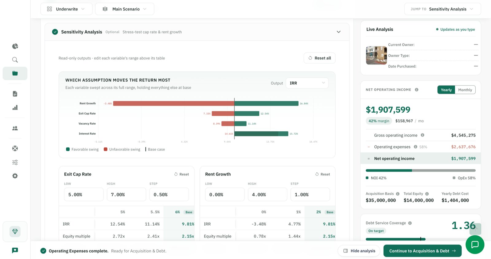
- One-variable sensitivity analysis on exit cap rate, rent growth, vacancy and interest rate, plus a two-variable grid on exit cap rate and income growth together.
- Property-tax reassessment modeling, and an explicit setting for whether replacement reserves sit above or below NOI — the convention that Step 3 spent a table on.
- Syndication and investor-split modeling, including preferred return, waterfall tiers and sponsor fees.
- Market context assembled from federal sources: Census demographic and housing data, Bureau of Labor Statistics employment data, and HUD Fair Market Rents. This data is cached — up to seven days for provider responses and 24 hours for the assembled market view — so treat it as a recent reference rather than a live feed.
- Notes, documents, reports and PDF export, so the assumptions behind an offer are written down and reviewable rather than living in one person's working file.
- Team collaboration on the top plan tier, with per-deal access control.
Capability availability depends on your plan: basic underwriting is available on every tier, while document import, multiple scenarios, scenario comparison, investor splits, refinance modeling and advanced reports require a higher tier, and team collaboration is on the top tier only. Some parts of the application are gated behind configuration and may not be enabled for your account.
One deliberate omission: an earlier, simplified underwriting mode has been deprecated and is now read-only. New analysis uses the detailed flow described above, and deals created in the old mode can be converted into it. If you have read about that mode elsewhere on this site or in older material, that is why it is not described here.
Work through this method on a property you are actually considering. Import the T12 and rent roll, set your own assumptions, and compare scenarios in one place.
Analyze a deal →What no software can verify for you
This list matters more than the one above it. Every item here is an input that the model treats as true, and none of them can be checked by any underwriting platform — DealWorthIt included. A model with excellent arithmetic and one wrong input produces a confident wrong answer.
- Physical condition. Whether the roof has five years left or one. That is a property condition assessment and a set of trade inspections, not a data feed.
- Whether the seller's documents are accurate. A rent roll is an assertion. Verifying it means reading the leases and tying the ledger to bank deposits.
- Whether the leases are enforceable, correctly executed, and consistent with what the rent roll claims they say.
- Environmental condition. Soil, tanks, asbestos, lead, mold, radon. A Phase I is a document you commission.
- Title. Liens, easements, encroachments, restrictive covenants, and whether the seller can actually convey.
- Zoning and legal use. Whether all 24 units are legally permitted, and whether the property is conforming or grandfathered — which decides what you may rebuild after a loss.
- Insurance availability and cost. Whether a carrier will write the risk at all, at what deductible, and with what exclusions. In some markets this now decides deals.
- Whether a market rent is actually achievable. A comparable property's asking rent is not proof that your renovated unit will lease at it, to a tenant who qualifies, without a concession.
- Whether a contractor's estimate is reliable, whether the scope is complete, and whether the schedule survives contact with a 1978 building.
- Property-tax reassessment. Modeling a reassessment is arithmetic; knowing your jurisdiction's actual rule, timing and appeal process is not.
- Whether the investment suits you. Your liquidity, tax position, risk capacity, time and experience are not model inputs.
- What the market does next. No dataset forecasts rent growth, cap rates or the cost of debt five years out. Anything presenting itself as such is an assumption wearing a chart.
Frequently asked questions
How do you underwrite a $2 million multifamily property?
Rebuild the income from the rent roll, normalize the T12 to your ownership costs, calculate in-place NOI on a stated convention, test what a lender will lend against that NOI, project operations you can defend, calculate the returns on the resulting equity, stress-test every material assumption, and compare the outcome to return requirements you set before you saw the deal. The price is the output of that process, not its input.
What should investors check in a rent roll?
Current rent against market rent unit by unit, occupied versus merely leased units, physical versus economic occupancy, delinquency by unit rather than in aggregate, concessions and whether they recur, lease expiration concentration, month-to-month tenancies, employee and model units, down units that are capital rather than vacancy, the unit mix against actual demand, and total loss to lease. In the example above, physical occupancy of 87.5% corresponds to economic occupancy of 75.7%.
How do you normalize a T12?
Adjust each line from what the seller spent to what you will spend, and document why. The lines that most often move: property taxes after reassessment, insurance at a current quote, management at market cost even when self-managing, repairs and maintenance to a sustainable per-unit level, and payroll where an owner's unpaid labor appears nowhere. Also separate recurring income from one-time income, and recurring expenses from capital.
How is multifamily NOI calculated?
Effective gross income less operating expenses. Effective gross income is gross potential rent less loss to lease, vacancy, concessions and credit loss, plus other income. Operating expenses exclude debt service and capital expenditure. Whether replacement reserves sit above or below the NOI line is a convention you must state — this article puts them below, and reports a separate lender-basis NOI with the reserve netted out.
What is DSCR?
Debt service coverage ratio: NOI divided by annual debt service. At 1.25x the property generates 25% more NOI than its mortgage payments require. Below 1.00x it does not cover them at all. Which NOI you use changes the answer, so lender-basis and investor-basis DSCR should always be labeled — in the example above the same loan produces 0.97x on one basis and 0.91x on the other.
What is debt yield?
NOI divided by the loan amount: a measure of how much property income stands behind each dollar lent, independent of the interest rate and amortization — so unlike DSCR it cannot be flattered by cheap debt or a 40-year schedule. It is a credit-risk ratio, not a foreclosure-recovery estimate; what a lender would actually recover depends on costs, timing and the property's value at that point. In the example above, an 8% minimum debt yield is one of the three caps used to size the loan.
How do interest rates affect a multifamily acquisition?
Through two channels that partly offset each other when loan sizing is coverage-constrained: a lower rate does not simply reduce the payment — it also raises the loan the property can carry, so more of the purchase is debt-financed. In the hypothetical example above, moving from 7.75% to 5.75% raised the sized loan from $855,000 to $1,050,000 but moved the IRR less than a point, because the deal was coverage-constrained at both rates. How much rate matters in any real deal depends on which constraint binds.
How do you calculate break-even occupancy?
Divide total obligations by the revenue base, and state both. The convention used here is (operating expenses + replacement reserves + annual debt service) ÷ gross potential income, with all operating expenses treated as fixed. It produces an economic break-even, not a door count — because rents differ by unit type, no single number of occupied units corresponds to a break-even percentage. In the example, 71.0% at the sized loan and 79.7% at the loan originally requested.
What assumptions should be stress-tested?
At minimum: purchase price, interest rate, rent growth, vacancy, operating expenses, capital expenditure and exit cap rate. In this example, price, rent growth and exit cap rate moved the outcome most; interest rate moved it least, because loan sizing absorbed part of the change. Which variables dominate differs by deal, which is the reason to test rather than assume.
Can DealWorthIt decide whether a property is a good investment?
No. DealWorthIt organizes your inputs, applies stated conventions consistently, calculates the metrics, and lets you compare scenarios and test sensitivities. It cannot verify that the seller's documents are true, inspect the building, confirm that a market rent is achievable, price your risk, or know your circumstances. Every assumption in a model is a decision someone made, and the investment decision belongs to you and your advisers — not to the software.
Methodology and formulas
Every figure in this article is computed at full double precision and rounded only for display: money to whole dollars, rates to one decimal place unless stated, and coverage ratios and multiples to two decimals. One consequence worth naming: re-deriving a figure from the rounded numbers printed above it can differ from the figure shown by a few dollars, because the calculation used the unrounded value. The sale price is the clearest case — $171,767 ÷ 7.00% gives $2,453,814, four dollars below the $2,453,818 computed from the unrounded Year-5 NOI. The calculation is not performed in the article; it is performed by a standalone model that the site's test suite re-runs against these published assumptions on every build, so a figure here and the arithmetic behind it cannot diverge unnoticed.
| Measure | Formula |
|---|---|
| Gross potential rent | Σ (units × market rent × 12), all units |
| Loss to lease | Σ (occupied units × (market rent − lease rent) × 12) |
| Vacancy loss | Σ (vacant units × market rent × 12) |
| Effective rental income | GPR − loss to lease − vacancy − concessions − credit loss |
| Effective gross income | Effective rental income + other income |
| Investor-basis NOI | EGI − operating expenses (incl. property management, excl. reserves) |
| Lender-basis NOI | Investor-basis NOI − replacement reserves |
| Operating expense ratio | Operating expenses ÷ EGI |
| Cap rate | NOI ÷ purchase price (state which NOI) |
| Monthly debt service | Loan × r ÷ (1 − (1 + r)^−n), r = annual rate ÷ 12, n = months |
| DSCR | NOI ÷ annual debt service (state which NOI) |
| Debt yield | NOI ÷ loan amount (state which NOI) |
| Maximum loan by DSCR | NOI ÷ minimum DSCR ÷ annual constant per dollar of loan |
| Maximum loan by debt yield | NOI ÷ minimum debt yield |
| Total project cost | Price + closing costs + capital budget + financing fees + funded reserves |
| Total cash required | Total project cost − loan proceeds |
| Cash flow after debt service | NOI − replacement reserves − annual debt service |
| Cash-on-cash return | Cash flow after debt service ÷ total cash required |
| Break-even occupancy | (Operating expenses + reserves + debt service) ÷ gross potential income |
| Sale price | Trailing final-year NOI ÷ exit cap rate |
| Net sale proceeds | Sale price − selling costs − loan payoff balance |
| Levered cash flows | [−equity, CF₁ … CF₄, CF₅ + net sale proceeds] |
| IRR | The rate at which Σ CFₜ ÷ (1 + rate)^t = 0 |
| Equity multiple | Total distributions ÷ total equity |
| Total return on equity | Equity multiple − 1 (undiscounted, not annualized) |
Sources
No source is cited for any assumption in this article, because every assumption is invented. Sources are listed only for the external references made above, and are primary in each case:
- U.S. Department of the Treasury — Daily Treasury Par Yield Curve Rates. The par yield curve DealWorthIt reads for Treasury benchmarks.
- Federal Reserve Bank of New York — Reference Rates (SOFR, EFFR). The overnight and averaged secured rates, and the unsecured effective federal funds rate.
- Federal Reserve Bank of St. Louis — FRED. Used as a documented fallback source for the same series.
- U.S. Census Bureau — American Community Survey. Demographic and housing data behind the market context views.
- U.S. Bureau of Labor Statistics — Local Area Unemployment Statistics. Employment data behind the same views.
- U.S. Department of Housing and Urban Development — Fair Market Rents. HUD's published rent standards, used as a reference point rather than a market rent.
Disclaimer
This article is educational content published by DealWorthIt. The property, its operating history, the rent roll, the trailing twelve-month statement, the capital plan, the loan terms, the investor and every result are hypothetical and were created for teaching. They do not describe any real property, transaction, customer, lender or outcome, and they are not representative of results any user has obtained or should expect.
Nothing here is investment, tax, legal, accounting or lending advice. The loan terms are not an offer of credit and no lender has reviewed them. The example investor targets are illustrative and are not recommendations. Real estate investment involves risk, including the loss of principal. Consult qualified professionals about your own circumstances before acting on anything in this article.
DealWorthIt makes no guarantee of accuracy, completeness, savings, returns or outcomes. Analysis software calculates what it is told to calculate; the assumptions, the verification and the investment decision remain yours.
Ready to analyze your next deal?
Find, research, analyze, compare, and present real estate deals with DealWorthIt.
Related workflow in DealWorthIt: Multifamily
← Back to all articles